Tutorial : Computing ideal line profiles

In this tutorial you will, hopefully, learn how to compute ideal line Lyman-alpha line profiles with zELDA. The lines computed in this tutorial are ideal becase they don’t suffer from the typical artifacts caused by the fact the instruments are not perfect. These lines are in the rest frame of the galaxy.

Computing an ideal line profile

Let’s start by loading zELDA and setting the location of the LyaRT grids:

import Lya_zelda_II as Lya

your_grids_location = '/This/Folder/Contains/The/Grids/'

Lya.funcs.Data_location = your_grids_location

where /This/Folder/Contains/The/Grids/ is the place where you store the LyaRT data grids, as shown in the installation section.

Now, let’s decide which outflow geometry we want to use. For this tutorial we will use the gas geometry known as Thin Shell in which the intrinsic continuum is a gaussian and a continuum with a give equivalent width.

Geometry = 'Thin_Shell_Cont'

Let’s load the data containing the grid:

LyaRT_Grid = Lya.load_Grid_Line( Geometry )

This contains all the necessary information to compute the line profiles. To learn more about the grids of line profiles go to Installation . Remeber that if you want to use the line profile grid with lower RAM memory occupation you must pass MODE=’LIGHT’ to Lya.load_Grid_Line.

Now let’s define the parameters of the shell model that we want. these are five:

V_Value     = 50.0  # Outflow expansion velocity [km/s]
logNH_Value = 20.   # Logarithmic of the neutral hydrogen column density [cm**-2]
ta_Value    = 0.01  # Dust optical depth
logEW_Value = 1.5   # Logarithmic the intrinsic equivalent width [A]
Wi_Value    = 0.5   # Intrinsic width of the line [A]

Now, let’s set the wavelength array where we want to put the line in the international system of units (meters). We arbitrarily chose to evaluate the line +-10A around Lyman-alpha:

import numpy as np
w_Lya = 1215.68 # Lyman-alpha wavelength in amstrongs
wavelength_Arr = np.linspace( w_Lya-10 , w_Lya+10 , 1000 ) * 1e-10

Now he have everything, let’s compute the line simply by doing:

Line_Arr = Lya.RT_Line_Profile_MCMC( Geometry , wavelength_Arr , V_Value , logNH_Value , ta_Value , LyaRT_Grid , logEW_Value=logEW_Value , Wi_Value=Wi_Value )

And… It’s done! Line_Arr is a numpy array that contains the line profile evaluated in wavelength_Arr.

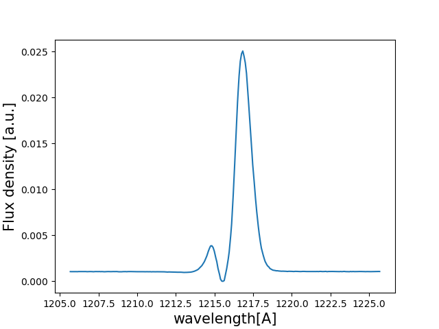
Let’s plot the line by doing

import pylab as plt
plt.plot( wavelength_Arr *1e10 , Line_Arr )
plt.xlabel('wavelength[A]' , size=15 )
plt.ylabel('Flux density [a.u.]' , size=15 )
plt.show()

This should show something like this

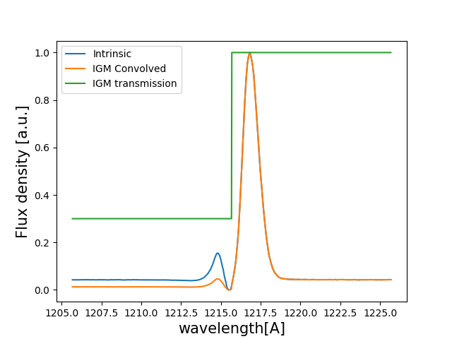
Computing an ideal line profile with the IGM absorption

Now let’s create an IGM transmission curve. This is a simple toy model. For this example we are going to set the IGM transmission bluer than Lyman-alpha to 0.3 and for redder than Lyman-alpha to 1.

w_Lya = 1215.68
T_IGM_Arr = np.ones( len( wavelength_Arr ) )

T_IGM_Arr[ wavelength_Arr * 1e10 < w_Lya ] = 0.3

Now let’s convolve the line profile with the IGM transmission curve

IGM_Line_Arr = Line_Arr * T_IGM_Arr

Let’s see how it looks

plt.plot( wavelength_Arr *1e10 , Line_Arr    *1./np.amax( Line_Arr )  , label='Intrinsic' )
plt.plot( wavelength_Arr *1e10 , IGM_Line_Arr*1./np.amax( Line_Arr )  , label='IGM Convolved' )
plt.plot( wavelength_Arr *1e10 , T_IGM_Arr , label='IGM transmission' )
plt.xlabel('wavelength[A]' , size=15 )
plt.ylabel('Flux density [a.u.]' , size=15 )
plt.legend(loc=0)
plt.show()

It should look something like this

Computing many ideal line profiles

Above we have just seen how to compute one ideal line profile. In the case that you want to compute several zELDA has a more compact function.

Let’s start like in the case above in which we set the location of the grids:

import Lya_zelda_II as Lya

your_grids_location = '/This/Folder/Contains/The/Grids/'

Lya.funcs.Data_location = your_grids_location

where /This/Folder/Contains/The/Grids/ is the place where you store the LyaRT data grids, as shown in the installation section.

Now, let’s set the geometry:

Geometry = 'Thin_Shell_Cont'

And now, instead of loading the grid, let’s define the outflow parameters. In this case they will be lists (or numpy arrays) as we want, for example 3 line profile configurations:

V_Arr     = [ 50.0 , 100.   , 200.    ] # Outflow expansion velocity [km/s]
logNH_Arr = [ 18.  ,  19.   ,  20.    ] # Logarithmic of the neutral hydrogen column density [cm**-2]
ta_Arr    = [  0.1 ,   0.01 ,   0.001 ] # Dust optical depth
logEW_Arr = [  1.  ,   1.5  ,   2.0   ] # Logarithmic the intrinsic equivalent width [A]
Wi_Arr    = [  0.1 ,   0.5  ,   1.0   ] # Intrinsic width of the line [A]

and the wavelength array

import numpy as np
w_Lya = 1215.68 # Lyman-alpha wavelength in amstrongs
wavelength_Arr = np.linspace( w_Lya-10 , w_Lya+10 , 1000 ) * 1e-10

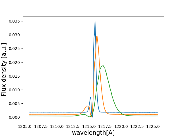
Now let’s actually compute the lines:

Line_Matrix = Lya.RT_Line_Profile( Geometry , wavelength_Arr , V_Arr , logNH_Arr , ta_Arr , logEW_Arr=logEW_Arr , Wi_Arr=Wi_Arr )

Line_Matrix is a 2-D numpy array containing the line profiles for the configurations. For example, Line_Matrix[0] has outflow velocity V_Arr[0], neutral hydrogen column density logNH_Arr[0] and so on.

Let’s plot them:

import pylab as plt

for i in range( 0 , 3 ) :
    plt.plot( wavelength_Arr *1e10 , Line_Matrix[i] )

plt.xlabel('wavelength[A]'       , size=15 )
plt.ylabel('Flux density [a.u.]' , size=15 )
plt.show()

This should show something like this:

Now you know how to get ideal Lyman-alpha line profiles!