Tutorial : Fitting a line profile using deep learning
In this tutorial you will, hopefully, learn how fit Lyman-alpha line profiles using deep learning with zELDA.
Getting started
Let’s start by loading zELDA creating a mock line profile that we will fit later. For more details on how to create a mock line profile go to Mock line profiles
import Lya_zelda_II as Lya
your_grids_location = '/This/Folder/Contains/The/Grids/'
Lya.funcs.Data_location = your_grids_location

Geometry = 'Thin_Shell_Cont'
LyaRT_Grid = Lya.load_Grid_Line( Geometry )

# Defining the model parameters:
z_t      = 0.5   # redshift of the source
V_t      = 50.0  # Outflow expansion velocity [km/s]
log_N_t  = 20.   # Logarithmic of the neutral hydrogen column density [cm**-2]
t_t      = 0.01  # Dust optical depth
log_EW_t = 1.5   # Logarithmic the intrinsic equivalent width [A]
W_t      = 0.5   # Intrinsic width of the line [A]
F_t      = 1.    # Total flux of the line

# Defining the quality of the line profile:
PNR_t  = 15.0 # Signal to noise ratio of the maximum of the line.
FWHM_t = 0.2  # Full width half maximum diluting the line. Mimics finite resolution. [A]
PIX_t  = 0.1  # Wavelength binning of the line. [A]

w_Arr , f_Arr , s_Arr = Lya.Generate_a_real_line( z_t , V_t, log_N_t, t_t, F_t, log_EW_t, W_t , PNR_t, FWHM_t, PIX_t, LyaRT_Grid, Geometry )
where /This/Folder/Contains/The/Grids/ is the place where you store the LyaRT data grids, as shown in the installation section. And… It’s done! w_Arr is a numpy array that contains the wavelength where the line profile is evaluated. Meanwhile, f_Arr is the actual line profile. s_Arr is the uncertainty of the flux density. Remeber that if you want to use the line profile grid with lower RAM memory occupation you must pass MODE=’LIGHT’ to Lya.load_Grid_Line.
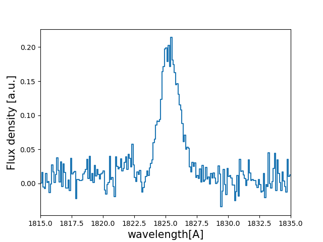
Let’s have a look to how the line looks:
w_Arr , f_Arr , s_Arr  = Lya.Generate_a_real_line( z_t , V_t, log_N_t, t_t, F_t, log_EW_t, W_t , PNR_t, FWHM_t, PIX_t, LyaRT_Grid, Geometry )

w_pix_Arr , f_pix_Arr = Lya.plot_a_rebinned_line( w_Arr , f_Arr , PIX_t )

import pylab as plt
plt.plot( w_pix_Arr , f_pix_Arr )
plt.xlabel('wavelength[A]' , size=15 )
plt.ylabel('Flux density [a.u.]' , size=15 )
plt.xlim(1815,1835)
plt.show()
Now that we have our mock line profile. Let’s load the neural network. As we have produce a line profile for an outflow (V_t>0) we are going to load the deep neural network for outflows
machine_data = Lya.Load_NN_model( 'Outflow' )
In case you want to do the analysis for inflows just call Lya.Load_NN_model( ‘Inflow’ ). machine_data is a python dictionary that contains all the necessary data for the deep neural network approach. Let’s pick up from it two variables:
machine    = machine_data['Machine' ]
w_rest_Arr = machine_data[ 'w_rest' ]
machine is an object from skitlearn with the trained neural network and w_rest_Arr is the rest frame wavelength where the line profiles used for the training were evaluated. w_rest_Arr is important to check that the neural networks is working in the same wavelength array that the line profiles will be evaluated. In principle you don’t have to do anything with w_rest_Arr, but we need to pass it to other functions.
Using the DNN in the un-perturbed line profile
Let’s start by simple evaluating the DNN using the mock line profile without perturbing it:
Sol , z_sol = Lya.NN_measure( w_Arr , f_Arr , s_Arr , FWHM_t , PIX_t , machine , w_rest_Arr , N_iter=None )
Done! . Sol is a matrix that contains the prediction by the DNN and z_sol is the predicted redshift. You can print the predicted properties doing:
print( 'The measured redshift                                                     is' , z_sol    )
print( 'The measured logarithm of the expasion velocity                           is' , Sol[0,1] )
print( 'The measured logarithm of the HI column density                           is' , Sol[0,2] )
print( 'The measured logarithm of the dust optical depth                          is' , Sol[0,3] )
print( 'The measured logarithm of the intrinsic equivalent width                  is' , Sol[0,4] )
print( 'The measured logarithm of the intrinsic            width                  is' , Sol[0,5] )
print( 'The measured shift of the true Lya wavelgnth from the maximum of the line is' , Sol[0,0] )
This should give something like
The measured redshift                                                     is 0.49994403239322693
The measured logarithm of the expasion velocity                           is 1.5821419036064905
The measured logarithm of the HI column density                           is 20.149247231711733
The measured logarithm of the dust optical depth                          is -3.310662004999448
The measured logarithm of the intrinsic equivalent width                  is 1.458352960574508
The measured logarithm of the intrinsic            width                  is -0.804093047888869
The measured shift of the true Lya wavelgnth from the maximum of the line is -1.2773994188976223
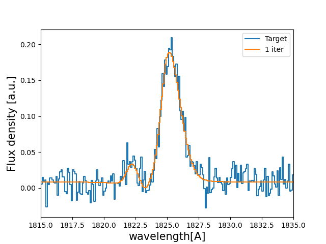
Let’s see how this new spectrum compares with the target:
PNR = 100000. # let's put infinite signal to noise in the model line

V_sol    = 10**Sol[0,1] # Expansion velocity km/s
logN_sol =     Sol[0,2] # log of HI column density cm**-2
t_sol    = 10**Sol[0,3] # dust optical depth
logE_sol =     Sol[0,4] # log intrinsic EW [A]
W_sol    = 10**Sol[0,5] # intrinsic width [A]

# creates the line

w_One_Arr , f_One_Arr , _  = Lya.Generate_a_real_line( z_sol , V_sol, logN_sol, t_sol, F_t, logE_sol, W_sol, PNR, FWHM_t, PIX_t, LyaRT_Grid, Geometry )

# plot the target and the predicted line

w_pix_One_Arr , f_pix_One_Arr = Lya.plot_a_rebinned_line( w_One_Arr , f_One_Arr , PIX_t )

plt.plot( w_pix_Arr     , f_pix_Arr     , label='Target' )
plt.plot( w_pix_One_Arr , f_pix_One_Arr , label='1 iter' )

plt.legend(loc=0)
plt.xlabel('wavelength[A]' , size=15 )
plt.ylabel('Flux density [a.u.]' , size=15 )
plt.xlim(1815,1835)
plt.show()
You should get something like:
Using the DNN with Monte Carlo perturbations
Normally, it is better to do more than one iteration, as it leads to better results. These iterations basically perturb the flux density f_Arr by adding gaussian noise with the amplitude of s_Arr in each wavelength bin. Then, this new perturbed spectrum is send to the DNN. For each of these iterations the output of the DNN is stored. For example for 1000 iterations :
>>> Sol , z_sol , log_V_Arr , log_N_Arr , log_t_Arr , z_Arr , log_E_Arr , log_W_Arr = Lya.NN_measure( w_Arr , f_Arr , s_Arr , FWHM_t , PIX_t , machine , w_rest_Arr , N_iter=1000 )
The arrays log_V_Arr, log_N_Arr, log_t_Arr, z_Arr, log_E_Arr and log_W_Arr contain the output of the DNN for the iterations for the logarithms of the expansion velocity, the logarithm of the neutral hydrogen column density, the logarithm of the dust optical depth, the redshift, the logarithm of the intrinsic equivalent width and the logarithm of the intrinsic width of the line. From these arrays we can compute the result from the DNN analysis by taking the 50th percentile. The +-1 sigma uncertainty can be computed as the 16th and 84th percentile.
import numpy as np

# Redshitft
z_50     = np.percentile(    z_Arr , 50 )
z_16     = np.percentile(    z_Arr , 16 )
z_84     = np.percentile(    z_Arr , 84 )

# Expansion velocity
V_50     = 10 ** np.percentile( log_V_Arr , 50 )
V_16     = 10 ** np.percentile( log_V_Arr , 16 )
V_84     = 10 ** np.percentile( log_V_Arr , 84 )

# Logarithmic of HI column density
log_N_50 = np.percentile( log_N_Arr , 50 )
log_N_16 = np.percentile( log_N_Arr , 16 )
log_N_84 = np.percentile( log_N_Arr , 84 )

# Dust optical depth
t_50     = 10 ** np.percentile( log_t_Arr , 50 )
t_16     = 10 ** np.percentile( log_t_Arr , 16 )
t_84     = 10 ** np.percentile( log_t_Arr , 84 )

# Logarithmic of intrinsic equivalent width
log_E_50 = np.percentile( log_E_Arr , 50 )
log_E_16 = np.percentile( log_E_Arr , 16 )
log_E_84 = np.percentile( log_E_Arr , 84 )

# Intrinsic width
W_50     = 10 ** np.percentile( log_W_Arr , 50 )
W_16     = 10 ** np.percentile( log_W_Arr , 16 )
W_84     = 10 ** np.percentile( log_W_Arr , 84 )
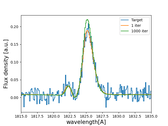
let’s see how the line profiles look:
# Compute the 100 iterations line profile
w_50th_Arr , f_50th_Arr , _  = Lya.Generate_a_real_line( z_50 , V_50, log_N_50, t_50, F_t, log_E_50, W_50, PNR, FWHM_t, PIX_t, LyaRT_Grid, Geometry )

# Get cooler profiles
w_pix_50th_Arr , f_pix_50th_Arr = Lya.plot_a_rebinned_line( w_50th_Arr , f_50th_Arr , PIX_t )

# Plot
plt.plot( w_pix_Arr      , f_pix_Arr      , label='Target'   )
plt.plot( w_pix_One_Arr  , f_pix_One_Arr  , label='1 iter'   )
plt.plot( w_pix_50th_Arr , f_pix_50th_Arr , label='1000 iter')

plt.legend(loc=0)
plt.xlabel('wavelength[A]' , size=15 )
plt.ylabel('Flux density [a.u.]' , size=15 )
plt.xlim(1815,1835)
plt.show()
finally, let’s compare the parameters that we got with the input:
print( 'The true redshift                 is' , z_t      , 'and the predicted is' , z_50     , '(-' , z_50-z_16         , ', +' , z_84-z_50         , ')' )
print( 'The true expansion velocity       is' , V_t      , 'and the predicted is' , V_50     , '(-' , V_50-V_16         , ', +' , V_84-V_50         , ')' )
print( 'The true dust optical depth       is' , t_t      , 'and the predicted is' , t_50     , '(-' , t_50-t_16         , ', +' , t_84-t_50         , ')' )
print( 'The true intrinsic width          is' , W_t      , 'and the predicted is' , W_50     , '(-' , W_50-W_16         , ', +' , W_84-W_50         , ')' )
print( 'The true log of HI column density is' , log_N_t  , 'and the predicted is' , log_N_50 , '(-' , log_N_50-log_N_16 , ', +' , log_N_84-log_N_50 , ')' )
print( 'The true log of equivalent width  is' , log_EW_t , 'and the predicted is' , log_E_50 , '(-' , log_E_50-log_E_16 , ', +' , log_E_84-log_E_50 , ')' )
This should give something like:
The true redshift                 is 0.5 and the predicted is 0.49999833428137275 (- 0.00017321665235831007 , + 0.0003615214512187048 )
The true expansion velocity       is 50.0 and the predicted is 47.070589157142614 (- 16.100374040796254 , + 48.27234502291723 )
The true dust optical depth       is 0.01 and the predicted is 0.00379679848371737 (- 0.003483235501588427 , + 0.049396128990436335 )
The true intrinsic width          is 0.5 and the predicted is 0.280484205908298 (- 0.12228181625600373 , + 0.2150273326940031 )
The true log of HI column density is 20.0 and the predicted is 20.019139948537997 (- 0.5728866241916535 , + 0.207985045834004 )
The true log of equivalent width  is 1.5 and the predicted is 1.5595962407058306 (- 0.09992888862396399 , + 0.16009784914990055 )
The particular values that you print will be slightly different when you run it, but more or less it should go in the same direction.
That was fun, hah? Now you know how to use the deep neural network scheme in zELDA.